Low Thrust 2D Orbital Trajectory Optimization

Ian Ruh

This originated as my final project for the Intro to Optimization course at UW Madison, with Prof. Stephen Wright.

The Jupyter notebook is available here.

using Pkg
Pkg.add("JuMP")
Pkg.add("PyPlot")
Pkg.add("Ipopt")

xxxxxxxxxx
using JuMP, PyPlot, Ipopt

1. Introduction

Since the first satellites were launched in the late 1950s, engineers and scientists have had to navigate the unfamiliar dynamics of orbital mechanics. The process of getting from point A to point B while in orbit is not an intuitive exercise for someone unfamiliar with how orbital mechanics works because it appears to disobey the laws of physics we are accustomed to in our everyday life.

For example, to launch a rocket, one may think that the objective is to go up so as to get into orbit; after all, the rockets are pointed directly vertical on the launch pads. Yet, the really important factor that determines whether you will stay in space once you have gotten there is how fast you are going sideways. Likewise, if you want to go from one orbit to another orbit, the most natural thing to do is point your rocket in that direction and hit the throttle (and hope any Kerbals get out or your way). That, however, is likely a very inefficient and resource intensive trajectory.

The problem of determining the most efficient way to get from one orbit to another is compounded by the variety of different propulsion systems used on different craft. On the low end (thrust-wise), we have solar sails that use the radiation pressure from the sun (or lasers on earth in some concepts) to alter their velocity. One such example was Mariner 3 (and 4) spacecrafts that used 4 'flaps' on the end of their solar panels to alter the surface area that was presented to the sun, and thus were able to use the radiation pressure for attitude control. Another more recent example is the Planetary Society's crowd-funded Light Sail 2 craft that was launched in 2019. Using a 32 square meter sail, it is able to get an acceleration of 0.058 $mm/s^2$$mm/s^2$. On the other end of the spectrum we have large chemical rockets in the ilk of the N1, Saturn V, and more recently, super heavy launch vehicles including Starship and New Glenn, which can produce millions of pounds of thrusts and launch multiple tons into LEO and beyond.

The most effective (and feasible) trajectories for these vehicles are drastically different. Both in terms of how large a thrust some can provide, and by the fact that most chemical combustion rocket engines have a minimum thrust that if gone below can damage the engine, while other propulsion technologies, including ion thrusters, have fairly low thrusts but can sustain them for very long periods of time.

In this project we look at two of the primary trade offs considered in determining trajectories in the context of a (relatively) low thrust propulsion system: time and fuel.

2. Mathematical Model

For the sake of tractability, the problem has been restricted to considering one body orbiting a much larger body (e.g. a satellite orbiting earth) in a single orbital plane. By limiting ourselves to a single plane, we are able to remove almost half of the orbital parameters that are typically used to define a 3D orbit around a body. Moreover, several additional factors are ignored, including (non-exhaustively) atmospheric effects, gravitational perturbations, and torques due to Earth's bulges.

By making these assumptions, we end up with the dynamics equations below:

$\dot{r}=v_r$$\dot{r} = v_r$

$\dot{\theta }=\frac{v_t}{r}$$\dot{\theta} = \frac{v_t}{r}$

$\dot{v_r}=\frac{v_t^2}{r}-\frac{\mu }{r^2}+usin(\varphi )$$\dot{v_r} = \frac{v_t^2}{r} - \frac{\mu}{r^2} + u\ sin(\phi)$

$\dot{v_t}=-\frac{v_t{v}_r}{r}+ucos(\varphi )$$\dot{v_t} = - \frac{v_t v_r}{r} + u\ cos(\phi)$

Where our state variables are radius ($r$$r$), phase ($\theta$$\theta$), radial velocity ($v_r$$v_r$), and tangential velocity ($v_t$$v_t$). And our control variables are thrust angle ($\varphi$$\phi$), and thrust magnitude ($u$$u$). One additional factor that we ignore is the change in mass as the craft's fuel is depleted.

One significant factor we have to consider here is the gravitational constant $\mu$$\mu$. In SI units, this has a value of $6.6743\cdot {10}^{-11}\frac{N\cdot m^2}{k{g}^2}$$6.6743\cdot 10^{-11} \frac{N\cdot m^2}{kg^2}$. However, we represent decimal numbers using floating point numbers, which lose accuracy at very small or very large scales. If we were to use SI units in our analysis, we would be multiplying a very small number (${10}^{-11}$$~10^{-11}$) by a very large number (the radius of the orbit in meters). This is a recipe for large numerical errors. Instead, we define the unit system we use such that the gravitational constant $\mu =1$$\mu = 1$. That way, all of the numbers we are dealing with remain on the order of magnitude of 1, where floating point numbers are the most dense, and thus retain the most accuracy.

Discretization

We also need to choose a method of discretizing our system. We initially show the results of using the simplest approach to our integration scheme in the first section below, and then proceed with using a much more accurate scheme.

The simplest scheme is forward Euler method where ${\int }_0^{1}f(x)\approx \frac{f(x_0)+f(x_1)}{2}\mathrm{\Delta }x$$\int_0^1f(x) \approx \frac{f(x_0) + f(x_1)}{2}\Delta x$. This is only a first order accurate scheme, though, and so has limited use for us as demonstrated in the next section.

However, there are many higher order schemes that we can use to increase the accuracy and stability of our model. The scheme we chose here is to use cubic Hermite interpolating polynomials, and integrate those over the domain from 0 to 1. Any cubic polynomial can be uniquely defined by four points, just as a quadratic can be uniquely defined by three, and a line by two. However, we can also uniquely define a cubic polynomial using only two points, and the values of the derivative of the polynomial at those points. The graphs below demonstrate this for several different cases.

​x
PyPlot.ioff()

"""
Utility to evaluate a given cubic hermite polynomial
"""
function hermitePolynomial(y0, y1, d0, d1)
    PyPlot.grid("on")
    f(t) = (2*t^3 - 3*t^2 + 1)*y0 + (t^3 - 2*t^2 + t)*d0 + (-2*t^3 + 3*t^2)*y1 + (t^3 - t^2)*d1
    xs = convert(Array, 0:0.01:1)
    fs = [f(x) for x in xs]
    PyPlot.plot(xs, fs)
    axis((0.0,1.0,-0.5,0.5));
    xlabel("x")
    ylabel("y")
end


fig = figure("pyplot_subplot_mixed",figsize=(8,8))
subplot(221)
PyPlot.title("y₀=-0.2, y₁=0.2, d₀=-1, d₁=1")
hermitePolynomial(-0.2, 0.2, -1, 1)
subplot(222)
PyPlot.title("y₀=0, y₁=0, d₀=1, d₁=-1")
hermitePolynomial(0, 0, 1, -1)
ax = subplot(223)
PyPlot.title("y₀=0, y₁=0, d₀=-1, d₁=-1")
hermitePolynomial(0, 0, -1, -1)
subplot(224)
PyPlot.title("y₀=1, y₁=-1, d₀=0, d₁=0")
hermitePolynomial(0.5, -0.5, 0, 0)
fig.canvas.draw() # Update the figure
fig.tight_layout()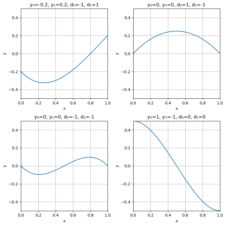

There are two primary reasons these polynomials are useful to us:

1. By having control over the derivatives of the polynomials at the end points we are able to make sure that all of our trajectories will be smooth. If the spacecraft in our model is moving at 10 m/s at the end of one segment, it shouldn't be moving at 11 m/s at the beginning of the next, as this would be an unrealistic discontinuity in the model.
2. The second reason is that it is very easy to integrate these polynomials. Because they are uniquely defined by the values and derivatives at the two endpoints, the integral over the polynomial from 0 to 1 is also easily expressed in terms of these values:

${\int }_0^1(2t^3-3t^2+1)y_0+(t^3-2t^2+t)\frac{dx}{dy}{|}_{x=0}+(-2t^3+3t^2)y_1+(t^3-t^2)\frac{dx}{dy}{|}_{x=1}dt=\frac{1}{2}{y}_0+\frac{1}{2}{y}_1+\frac{1}{12}\frac{dx}{dy}{|}_{x=0}-\frac{1}{12}\frac{dx}{dy}{|}_{x=1}$$\int_0^1 (2t^3 - 3t^2 + 1)y_0 + (t^3 - 2t^2 + t)\frac{dx}{dy}|_{x=0} + (-2t^3 + 3t^2)y_1 + (t^3 - t^2)\frac{dx}{dy}|_{x=1} dt = \frac{1}{2}y_0 + \frac{1}{2}y_1 + \frac{1}{12}\frac{dx}{dy}|_{x=0} - \frac{1}{12}\frac{dx}{dy}|_{x=1}$

$⟹{\int }_0^{1}f(t)dt\approx \frac{y_0}{2}+\frac{y_1}{2}+\frac{d_0}{12}-\frac{d_1}{12}$$\implies \int_0^1 f(t) dt \approx \frac{y_0}{2} + \frac{y_1}{2} + \frac{d_0}{12} - \frac{d_1}{12}$

Using this integration scheme we can achieve a much more accurate and stable system.

Problem Model

Our mathematical model for the fuel optimal problem is:

Where the constraints can be explained as follows:

• All radii should be positive, otherwise we have a degeneracy in our system.
• The thrust can only be positive, and is limited by some maximum thrust the engine can provide.
• The thrust angle can be arbitrarily limited to 0 to $2\pi$$2\pi$. However, this actually introduces a degeneracy some of the time. Throughout this notebook, you may notice that the thrust angle jumps from 0 to $2\pi$$2\pi$ in the middle of a trajectory. As both values are functionally equivalent, that has no physical meaning and is just a numerical artifact of the solution. Even applying a strict inequality constraint doesn't seem to alleviate this ambiguity.
• The initial radius is set.
• The initial tangential velocity is set.
• The initial radial velocity is set.
• The final radius is set.
• The final tangential velocity is set.
• The final radial velocity is set.

In addition, we have a series of N additional sets of constraints for the dynamics of the problem. Below is the first set of constraints for the dynamics, but they only change in the variable indexing for all other steps.

You may have guessed based on the dynamics constraints, but our optimization problem turns out to be non-linear.

3. Solution

Utility Functions

We first define some utility functions below.

xxxxxxxxxx
"""
A utility function to calculate the tangential velocity required to achieve a
circular orbit at a given altitude.
"""
function getCircularVelocity(r)
    return 1/sqrt(r)
end
getCV = getCircularVelocity

"""
A function to reconstruct the interpolated values of a cubic Hermite Polynomial
based on the endpoints and derivatives.
"""
function segmentInterp(y0, y1, d0, d1, n_per_segment)
    f(y0, y1, d0, d1, t) = (2*t^3 - 3*t^2 + 1)*y0 + (t^3 - 2*t^2 + t)*d0 + (-2*t^3 + 3*t^2)*y1 + (t^3 - t^2)*d1
    output = []
    times = []
    for i=1:n_per_segment
        time = i/n_per_segment
        push!(output, f(y0, y1, d0, d1, time))
        push!(times, time)
    end
    
    return (output, times)
end

"""
We utilize the linear interpolations for several non-state variables where it would not
be significantly beneficial to use a higher order method.
"""
function linInterp(y0, y1, n_per_segment)
    f(y0, y1, t) = (y1 - y0)*t + y0
    output = []
    times = []
    for i=1:n_per_segment
        time = i/n_per_segment
        push!(output, f(y0, y1, time))
        push!(times, time)
    end
    
    return (output, times)
end

"""
This function just reconstructs and interpolates the state
variables at a higher density than they are solved at.

It has no impact on the results and only serves to have the
orbit diagrams more closely reflect what the model is
solving.
"""
function reconstructPaths(n_per_segment=50; out_dis)
    N_original = length(out_dis["r"])
    out_interp = Dict()
    
    r_new = []
    θ_new = []
    vr_new = []
    vt_new = []
    ϕ_new = []
    u_new = []
    ar_new = []
    at_new = []
    time_new = []
    for i = 1:(N_original-1)
        (r_seg, time_seg) = segmentInterp(out_dis["r"][i], out_dis["r"][i+1], out_dis["vr"][i], out_dis["vr"][i+1], n_per_segment)
        (θ_seg, time_seg) = linInterp(out_dis["θ"][i], out_dis["θ"][i+1], n_per_segment)
        (vr_seg, time_seg) = linInterp(out_dis["vr"][i], out_dis["vr"][i+1], n_per_segment)
        (vt_seg, time_seg) = linInterp(out_dis["vt"][i], out_dis["vt"][i+1], n_per_segment)
        (ϕ_seg, time_seg) = linInterp(out_dis["ϕ"][i], out_dis["ϕ"][i+1], n_per_segment)
        (u_seg, time_seg) = linInterp(out_dis["u"][i], out_dis["u"][i+1], n_per_segment)
        (ar_seg, time_seg) = linInterp(out_dis["ar"][i], out_dis["ar"][i+1], n_per_segment)
        (at_seg, time_seg) = linInterp(out_dis["at"][i], out_dis["at"][i+1], n_per_segment)
        r_new = vcat(r_new, r_seg)
        θ_new = vcat(θ_new, θ_seg)
        vr_new = vcat(vr_new, vr_seg)
        vt_new = vcat(vt_new, vt_seg)
        ϕ_new = vcat(ϕ_new, ϕ_seg)
        u_new = vcat(u_new, u_seg)
        ar_new = vcat(ar_new, ar_seg)
        at_new = vcat(at_new, at_seg)
        time_new = vcat(time_new, time_seg .+ out_dis["t"][i])
    end
    
    return Dict(
        "r" => r_new,
        "θ" => θ_new,
        "vr" => vr_new,
        "vt" => vt_new,
        "ϕ" => ϕ_new,
        "u" => u_new,
        "ar" => ar_new,
        "at" => at_new,
        "t" => time_new
    )
    
end

"""
Given a solved trajectory, determine how long it takes to get to a given orbit.
"""
function timeToOrbit(outputs, r_final)
    r_delta = 0.01
    vt_delta = 0.01
    vr_delta = 0.01
    
    for i in 1:(size(outputs["t"])[1]-1)
        if(outputs["r"][i] < r_final + r_delta && outputs["r"][i] > r_final - r_delta &&
            outputs["vr"][i] < vr_delta && outputs["vr"][i] > -1*vr_delta &&
            outputs["vt"][i] < getCV(r_final) + vt_delta && outputs["vt"][i] > getCV(r_final) - vt_delta)
            return outputs["t"][i]
        end
    end
end

"""
Given a solved trajectory, determine how much fuel is used.
"""
function fuelUsed(outputs)
    total = 0.0
    
    for i in 1:(size(outputs["t"])[1]-2)
        total += outputs["u"][i]*(outputs["t"][i+1] - outputs["t"][i])
    end
    
    return total
end

"""
Given a solved trajectory, how many thrust segments were there.
"""
function thrustSegments(outputs)
    total = 0
    
    thrusting = false
    for i in 1:(size(outputs["t"])[1])
        if(outputs["u"][i] > 0.0005 && thrusting == false)
            thrusting = true
            total += 1
        elseif(outputs["u"][i] <= 0.0005 && thrusting == true)
            thrusting = false
        end
    end
    
    return total
end

First Order Method

In this example we demonstrate the limitations of using a first order accurate integration scheme. Refer to the comments for a description of what each line/section does.

xxxxxxxxxx
"""
This function builds and runs our model to optimize the orbital trajectory.

Parameters:
- r_init: The initial radius
- r_final: The final radius
- N: The number of segments to use
- T: The total time period to simulate for
"""
function transferOrbit(;r_init, r_final, N, T)
    # Model options
    μ = 1 # Gravitational constant
    max_thrust = 0.1 # Maximum thrust
    
    # Calculated values
    dt = T/N

    # Declare model
    model = Model()

    # Declare our models variables
    @variable(model, r[1:N] >= 0)   # Radius state variable
    @variable(model, θ[1:N])        # Phase state variable
    @variable(model, vr[1:N])       # Radial velocity state variable
    @variable(model, vt[1:N])       # Tangential velocity state variable
    
    @variable(model, ϕ[1:N])        # Thrust angle control variable
    @variable(model, u[1:N] >= 0)   # Thrust magnitude control variable
    
    # Initial Conditions (circular at an altitude of r_init)
    @constraint(model, r[1] == r_init)
    @constraint(model, θ[1] == 0)
    @constraint(model, vr[1] == 0)
    @constraint(model, vt[1] == getCV(r_init))
    
    # Misc Constraints
    @constraint(model, u .<= max_thrust)  # Limit the amount of thrust that can be provided
    @constraint(model, ϕ .<= 2*pi)
    @constraint(model, ϕ .>= 0)

    # Final state constraint (circular orbit at an altitude of r_final)
    @constraint(model, r[N] == r_final)
    @constraint(model, vr[N] == 0)
    @constraint(model, vt[N] == getCV(r_final))
    
    # Dynamics constraints
    for i in 2:N
        # Using just forward euler to integrate the state variables according to the dynamics equations
        @constraint(model,   r[i] - r[i-1] == dt*(vr[i-1]        + vr[i])      /2)
        @NLconstraint(model, θ[i] - θ[i-1] == dt*(vt[i-1]/r[i-1] + vt[i]/r[i]) /2)
        @NLconstraint(model, vr[i] - vr[i-1] == dt*(vt[i-1]^2/r[i-1] - μ/r[i-1]^2 + u[i-1]*sin(ϕ[i-1]) + vt[i]^2/r[i] - μ/r[i]^2 + u[i]*sin(ϕ[i])) /2)
        @NLconstraint(model, vt[i] - vt[i-1] == dt*(u[i-1]*cos(ϕ[i-1]) - vr[i-1]*vt[i-1]/r[i-1] + u[i]*cos(ϕ[i]) - vr[i]*vt[i]/r[i]) /2)

    end
    
    # Our objective is to change our orbit using the minimum amount
    # of fuel possible.
    @objective(model, Min, sum(u))
    
    # We set the optimizer  to use for the problem
    set_optimizer(model, with_optimizer(Ipopt.Optimizer));
    set_optimizer_attribute(model, "print_level", 3);
    optimize!(model)
    
    
    # Collect and return the model's variables
    r_final = value.(r)
    θ_final = value.(θ)
    vr_final = value.(vr)
    vt_final = value.(vt)
    
    ϕ_final = value.(ϕ)
    u_final = value.(u)
    
    return (r_final, θ_final, vr_final, vt_final, ϕ_final, u_final)
end

Now, after defining our model, we can run it. We look at a trajectory starting at a radius of two and raising it to three.

xxxxxxxxxx
(r_final, theta_final, vr_final, vt_final, phi_final, u_final) = transferOrbit(
    r_init = 2.0, # Initial orbit radius
    r_final = 3.0, # Final orbit radius
    N = 100, # Number of segments
    T = 12.0, # Total time period
)

xxxxxxxxxx
******************************************************************************
This program contains Ipopt, a library for large-scale nonlinear optimization.
 Ipopt is released as open source code under the Eclipse Public License (EPL).
         For more information visit http://projects.coin-or.org/Ipopt
******************************************************************************

Total number of variables............................:      600
                     variables with only lower bounds:      200
                variables with lower and upper bounds:        0
                     variables with only upper bounds:        0
Total number of equality constraints.................:      403
Total number of inequality constraints...............:      300
        inequality constraints with only lower bounds:      100
   inequality constraints with lower and upper bounds:        0
        inequality constraints with only upper bounds:      200

xxxxxxxxxx
Number of Iterations....: 275
                                   (scaled)                 (unscaled)
Objective...............:   1.2906157047443689e+00    1.2906157047443689e+00
Dual infeasibility......:   5.8214176803101869e-09    5.8214176803101869e-09
Constraint violation....:   2.7176964021227712e-14    2.7176964021227712e-14
Complementarity.........:   9.0912510740244202e-10    9.0912510740244202e-10
Overall NLP error.......:   5.8214176803101869e-09    5.8214176803101869e-09

xxxxxxxxxx
Number of objective function evaluations             = 437
Number of objective gradient evaluations             = 270
Number of equality constraint evaluations            = 437
Number of inequality constraint evaluations          = 437
Number of equality constraint Jacobian evaluations   = 296
Number of inequality constraint Jacobian evaluations = 296
Number of Lagrangian Hessian evaluations             = 275
Total CPU secs in IPOPT (w/o function evaluations)   =      3.830
Total CPU secs in NLP function evaluations           =      1.325

EXIT: Optimal Solution Found.

xxxxxxxxxx
fig = figure(figsize=(10,10)) # Create a new figure
ax = PyPlot.axes(polar="true") # Create a polar axis
PyPlot.title("Fuel Optimum Transfer Trajectory")
p = plot(theta_final,r_final,linestyle="-",marker="None") # Basic line plot

dtheta = 10
ax.set_thetagrids(collect(0:dtheta:360-dtheta)) # Show grid lines from 0 to 360 in increments of dtheta
ax.set_theta_zero_location("N") # Set 0 degrees to the top of the plot
ax.set_theta_direction(-1) # Switch to clockwise
fig.canvas.draw() # Update the figure

fig = figure("pyplot_subplot_mixed",figsize=(10,4))
subplot(221)
plot(u_final);
title("Thrust")
subplot(222)
plot(phi_final);
title("Thrust Angle")
subplot(223)
plot(vt_final);
title("Tangential Velocity")
subplot(224)
plot(vr_final);
title("Radial Velocity")
fig.canvas.draw() # Update the figure
fig.tight_layout()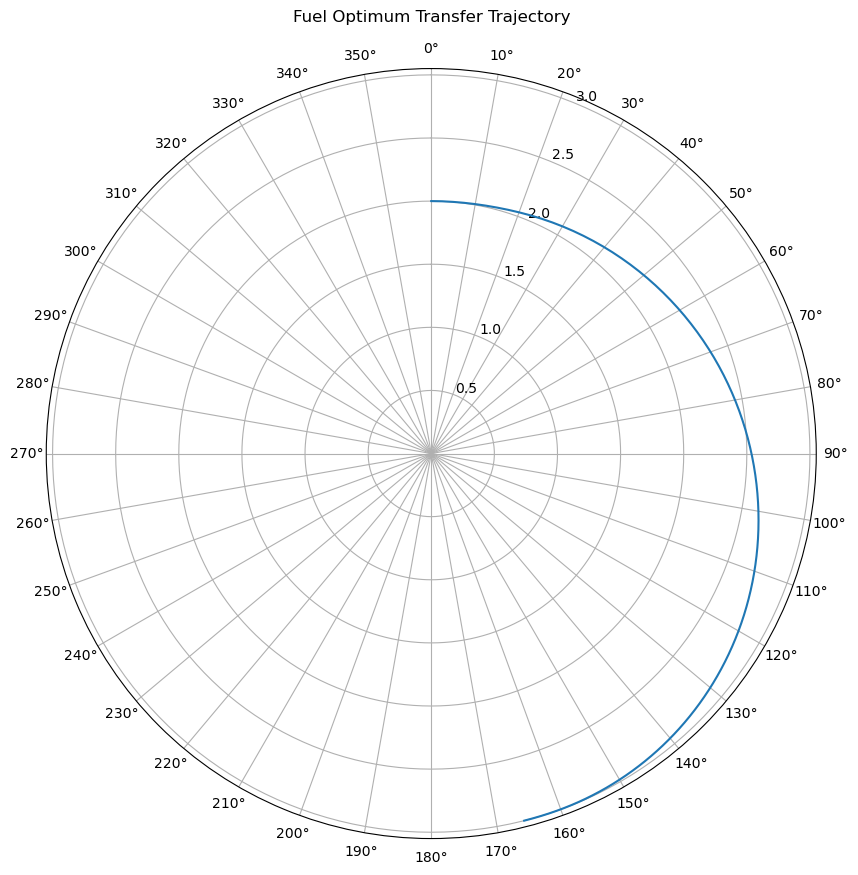

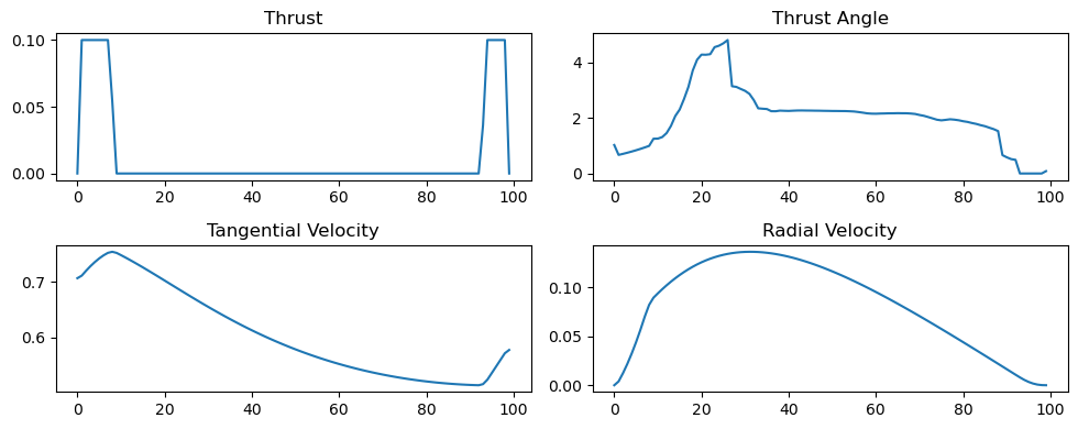
Saving some more in depth discussions of the results here for when we get more accurate trajectories in the next section, we'll just note a couple of items.

• The thrust angle graph looks weird. It is weird, because it is largely meaningless. The thrust angle is unconstrained by the model when the thrust is equal to zero, as it doesn't matter what direction your engine is pointing if it isn't turned on. Only the angles when the thrust is non-zero are physically relevant.
• Second, we can qualitatively compare this observed orbit to a Hohmann transfer, and immediately see the similarities. We start from a circular orbit, get into an elliptical orbit with an apoapsis at the level of our target orbit, then raise the periapsis when we get to the apoapsis.

Next, we'll demonstrate the instability in our current model by just increasing our simulation time a little bit. In the previous run, we used $N=100$$N=100$ and $T=12.0$$T=12.0$, so our time step was $\mathrm{\Delta }t\approx 0.12$$\Delta t \approx 0.12$. When numerically integrating a function, as we are doing in our model, the time step is one of the parameters that controls whether your scheme is stable. Large time steps, when coupled with fast dynamics, lead to significant error that can build up over the simulation lifetime and lead to meaningless results. If you decrease your time step, you can control that error, but at the cost of having to make more calculations to simulate the same time period. In this demonstration, we use a time step only slightly larger, at $\mathrm{\Delta }t\approx 0.16$$\Delta t \approx 0.16$.

xxxxxxxxxx
(r_final, theta_final, vr_final, vt_final, phi_final, u_final) = transferOrbit(
    r_init = 2.0, # Initial orbit radius
    r_final = 3.0, # Final orbit radius
    N = 100, # Number of segments
    T = 16.0, # Total time period
)

xxxxxxxxxx
Total number of variables............................:      600
                     variables with only lower bounds:      200
                variables with lower and upper bounds:        0
                     variables with only upper bounds:        0
Total number of equality constraints.................:      403
Total number of inequality constraints...............:      300
        inequality constraints with only lower bounds:      100
   inequality constraints with lower and upper bounds:        0
        inequality constraints with only upper bounds:      200

Number of Iterations....: 3000
                                   (scaled)                 (unscaled)
Objective...............:   5.3773910687749185e+00    5.3773910687749185e+00
Dual infeasibility......:   1.0478741122425304e+00    1.0478741122425304e+00
Constraint violation....:   2.0851140079821096e+00    3.1121554823118458e+03
Complementarity.........:   3.4364842033426444e-03    3.4364842033426444e-03
Overall NLP error.......:   2.0851140079821096e+00    3.1121554823118458e+03

Number of objective function evaluations             = 33821
Number of objective gradient evaluations             = 354
Number of equality constraint evaluations            = 33821
Number of inequality constraint evaluations          = 33821
Number of equality constraint Jacobian evaluations   = 3048
Number of inequality constraint Jacobian evaluations = 3048
Number of Lagrangian Hessian evaluations             = 3000
Total CPU secs in IPOPT (w/o function evaluations)   =     22.633
Total CPU secs in NLP function evaluations           =      7.238

EXIT: Maximum Number of Iterations Exceeded.

If you look at the output above closely, you'll see that the solver didn't actually converge to a solution. We can still look at its outputs though and see where it ended up:

xxxxxxxxxx
fig = figure(figsize=(10,10)) # Create a new figure
ax = PyPlot.axes(polar="true") # Create a polar axis
PyPlot.title("Unstable Transfer Trajectory")
p = plot(theta_final,r_final,linestyle="-",marker="None") # Basic line plot

dtheta = 10
ax.set_thetagrids(collect(0:dtheta:360-dtheta)) # Show grid lines from 0 to 360 in increments of dtheta
ax.set_theta_zero_location("N") # Set 0 degrees to the top of the plot
ax.set_theta_direction(-1) # Switch to clockwise
fig.canvas.draw() # Update the figure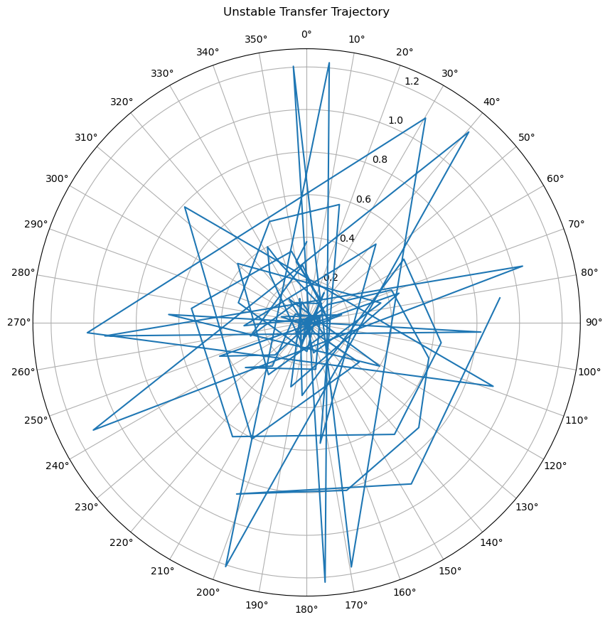

Clearly this doesn't seem likely to be a good prediction of reality. It probably also violates several laws of physics if we cared to do the math.

This is just to show the importance of the numerical scheme used in the model. In the next section we construct a very similar model, but use the higher order integration scheme described before, namely integrating cubic Hermite interpolating polynomials. Note the time steps we used above (on the order of $0.1$$0.1$) to the ones we can use below.

Hermite Interpolation

Below we construct the model using the integration scheme described in the introduction, and using a fuel optimal or a pseudo-time optimal objective function, which is discussed in the results section.

xxxxxxxxxx
@enum Objectives fuelOptimal pseudoTime

"""
Parameters:
- λ1 is the penalty parameter for the pseudo time optimal objective
- modelObjective chooses which objective function to use
- T is the total time horizon
- N is the number of nodes
- max_thrust is the maximum thrust that can be applied
- r_init is the initial orbit radius
- r_final is the final orbit radius
"""
function transferOrbitHermite(λ1; modelObjective, T, N, max_thrust, r_init, r_final)
    # Model options
    μ = 1 # Gravitational constant
    
    # Calculated values
    dt = T/N

    # Declare model
    model = Model()

    # Declare our models variables
    @variable(model, r[1:N] >= 0)
    @variable(model, θ[1:N])
    @variable(model, vr[1:N])
    @variable(model, vt[1:N])
    @variable(model, ar[1:N])
    @variable(model, at[1:N])
    
    @variable(model, ϕ[1:N])
    @variable(model, u[1:N] >= 0)
    
    # Slack variable for pseudo time optimal
    @variable(model, slackR[1:N])
    
    # Starting Values (starts everything in circular orbit at the initial altitude)
    set_start_value.(u, zeros(N))
    set_start_value.(ϕ, zeros(N))
    set_start_value.(r, r_init*ones(N))
    set_start_value.(vr, zeros(N))
    set_start_value.(vt, getCV(r_init)*ones(N))
    set_start_value.(ar, zeros(N))
    set_start_value.(at, zeros(N))
    
    # Initial Conditions (circular orbit at given radius)
    @constraint(model, r[1] == r_init)
    @constraint(model, θ[1] == 0)
    @constraint(model, vr[1] == 0)
    @constraint(model, vt[1] == getCV(r_init))
    
    # Misc Constraints
    @constraint(model, u .<= max_thrust)
    @constraint(model, ϕ .<= 2*pi - 1e-9) # Approximate strict inequality (doesn't really work)
    @constraint(model, ϕ .>= 0)

    # Final state constraint (circular orbit at given radius)
    @constraint(model, r[N] == r_final)
    @constraint(model, vr[N] == 0)
    @constraint(model, vt[N] == getCV(r_final))
    
    # Dynamics constraints
    @constraint(model, at[1] == (vt[2] - vt[1])/dt)
    @constraint(model, ar[1] == (vr[2] - vr[1])/dt)
    for i in 2:N
        # Indexing variables
        istart = i-1;
        iend = i;
        
        # Radial
        @constraint(model, r[iend] - r[istart] == dt*(vr[istart]/2 + vr[iend]/2 + ar[istart]/12 - ar[iend]/12))
        
        # Phase
        @NLconstraint(model, θ[iend] - θ[istart] == dt*(vt[istart]/r[istart]/2 + vt[iend]/r[iend]/2 + 1/12*(at[istart]/r[istart] - vt[istart]*vr[istart]/r[istart]^2) - 1/12*(at[iend]/r[iend] - vt[iend]*vr[iend]/r[iend]^2)))
        
        # Radial acceleration
        if(i < N)
            @constraint(model, ar[i] == (vr[i+1] - vr[i-1])/2/dt)
        elseif(i == N)
            @constraint(model, ar[i] == (vr[i] - vr[i-1])/dt)
        end
        
        # Radial Velocity
        @NLconstraint(model, vr[iend] - vr[istart] == dt*(
                (1/2)*(vt[istart]^2/r[istart] - μ/r[istart]^2+u[istart]*sin(ϕ[istart])) + 
                (1/2)*(vt[iend]^2/r[iend] - μ/r[iend]^2+u[iend]*sin(ϕ[iend])) + 
                (1/12)*(2*vt[istart]*at[istart]/r[istart] - vt[istart]^2*vr[istart]/r[istart]^2 + 2*μ/r[istart]^3*vr[istart] + (u[iend]-u[istart])/dt*sin(ϕ[istart]) + u[istart]*(ϕ[iend]-ϕ[istart])/dt*cos(ϕ[istart])) -
                (1/12)*(2*vt[iend]*at[iend]/r[iend] - vt[iend]^2*vr[iend]/r[iend]^2 + 2*μ/r[iend]^3*vr[iend] + (u[iend]-u[istart])/dt*sin(ϕ[iend]) + u[iend]*(ϕ[iend]-ϕ[istart])/dt*cos(ϕ[iend]))
        ))
        
        # Tangential acceleration
        if(i < N)
            @constraint(model, at[i] == (vt[i+1] - vt[i-1])/2/dt)
        elseif(i == N)
            @constraint(model, at[i] == (vt[i] - vt[i-1])/dt)
        end
        
        # Tangential Velocity
        @NLconstraint(model, vt[iend] - vt[istart] == dt*(
                (1/2)*(-1*vr[istart]*vt[istart]/r[istart] + u[istart]*cos(ϕ[istart])) +
                (1/2)*(-1*vr[iend]*vt[iend]/r[iend] + u[iend]*cos(ϕ[iend])) +
                (1/12)*(vr[istart]^2*vt[istart]/r[istart]^2 - (vr[istart]*at[istart]+ar[istart]*vt[istart])/r[istart] - u[istart]*sin(ϕ[istart])*(ϕ[iend]-ϕ[istart])/dt + (u[iend]-u[istart])/dt*cos(ϕ[istart])) -
                (1/12)*(vr[iend]^2*vt[iend]/r[iend]^2 - (vr[iend]*at[iend]+ar[iend]*vt[iend])/r[iend] - u[iend]*sin(ϕ[iend])*(ϕ[iend]-ϕ[istart])/dt + (u[iend]-u[istart])/dt*cos(ϕ[iend]))
        ))

    end
    
    # Slack constraints
    @constraint(model, slackR .>= r .- r_final)
    @constraint(model, slackR .>= -1(r .- r_final))
    
    # Choose the objective function
    if(modelObjective == fuelOptimal)
        @objective(model, Min, sum(u))
    elseif(modelObjective == pseudoTime)
        @objective(model, Min, sum(u) + λ1*sum(slackR))
    else
        # Default to fuel optimal
        @objective(model, Min, sum(u))
    end
    
    # Solve the problem
    set_optimizer(model, with_optimizer(Ipopt.Optimizer));
    set_optimizer_attribute(model, "print_level", 3);
    optimize!(model)
    
    # Output the results
    r_out = value.(r)
    θ_out = value.(θ)
    vr_out = value.(vr)
    vt_out = value.(vt)
    ar_out = value.(ar)
    at_out = value.(at)
    
    ϕ_out = value.(ϕ)
    u_out = value.(u)
    
    return Dict(
        "r" => r_out,
        "θ" => θ_out,
        "vr" => vr_out,
        "vt" => vt_out,
        "ϕ" => ϕ_out,
        "u" => u_out,
        "ar" => ar_out,
        "at" => at_out,
        "t" => convert(Array, 0:dt:T)
    )
end

xxxxxxxxxx
"""
This is simply a utility function to run a simulation and plot its outputs.
"""
function runHermite(plotTitle, λ1=0.0;modelObjective, T, N, max_thrust, r_init, r_final)
    output = transferOrbitHermite(
        λ1,
        modelObjective=modelObjective,
        T=T,
        N=N,
        max_thrust=max_thrust,
        r_init=r_init,
        r_final=r_final
    )
    
    output = reconstructPaths(out_dis=output)
    
    fig = figure(figsize=(10,10)) # Create a new figure
    ax = PyPlot.axes(polar="true") # Create a polar axis
    PyPlot.title(plotTitle)
    p = scatter(output["θ"][end:-1:1], output["r"][end:-1:1], c=output["u"][end:-1:1], cmap="jet", s=1.0)

    dtheta = 10
    ax.set_thetagrids(collect(0:dtheta:360-dtheta)) # Show grid lines from 0 to 360 in increments of dtheta
    ax.set_theta_zero_location("N") # Set 0 degrees to the top of the plot
    ax.set_theta_direction(-1) # Switch to clockwise
    ax[:set_yticks](convert(Array, 0:0.5:r_final+0.5))
    color_bar = PyPlot.colorbar()
    color_bar.set_label("Thrust")
    fig.canvas.draw() # Update the figure
    
    fig = figure("pyplot_subplot_mixed",figsize=(10,6))
    subplot(321)
    plot(output["t"], output["r"]);
    title("Radius")
    subplot(322)
    plot(output["t"], output["u"]);
    title("Thrust")
    subplot(323)
    plot(output["t"], output["ϕ"] .% (2*pi));
    title("Thrust Angle")
    subplot(324)
    plot(output["t"], output["vt"]);
    title("Tangential Velocity")
    subplot(325)
    plot(output["t"], output["vr"]);
    title("Radial Velocity")
    subplot(326)
    plot(output["t"], output["θ"]);
    title("Phase")
    fig.canvas.draw() # Update the figure
    suptitle("Transfer Orbit Profiles")
    fig.tight_layout()
end

Fuel Optimal

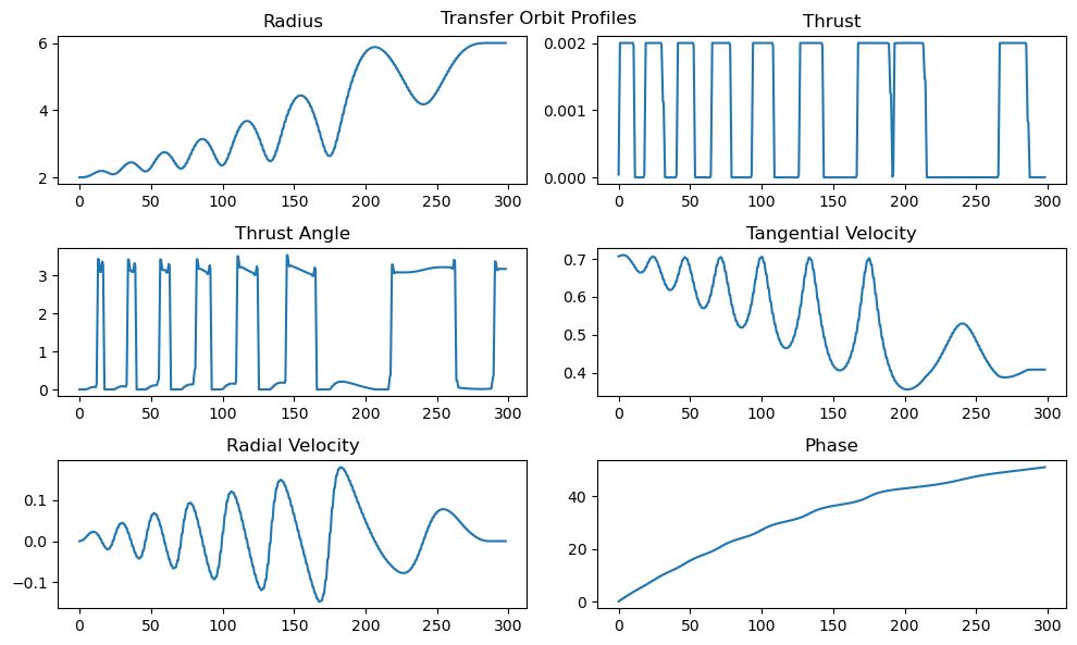
We do a fuel optimal transfer orbit from a height of 2 to a height of 6. Notice, we also use a time step of 1.5, 15 times larger than for the simple integration scheme, and this isn't even very close to the limit of the model's stability.

xxxxxxxxxx
runHermite(
    "Fuel Optimum Transfer Trajectory",
    modelObjective=fuelOptimal,
    T=300.0,
    N=200,
    max_thrust=0.002,
    r_init=2.0,
    r_final=6.0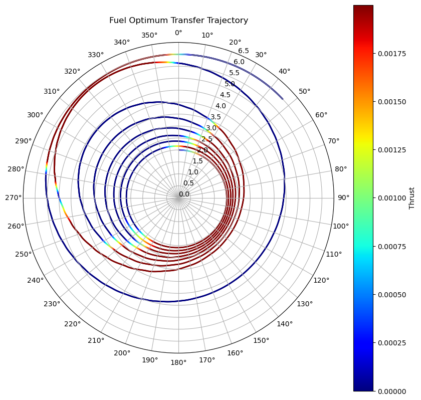
)

xxxxxxxxxx
Total number of variables............................:     1800
                     variables with only lower bounds:      400
                variables with lower and upper bounds:        0
                     variables with only upper bounds:        0
Total number of equality constraints.................:     1203
Total number of inequality constraints...............:     1000
        inequality constraints with only lower bounds:      600
   inequality constraints with lower and upper bounds:        0
        inequality constraints with only upper bounds:      400

Number of Iterations....: 165
                                   (scaled)                 (unscaled)
Objective...............:   1.9469062148290456e-01    1.9469062148290456e-01
Dual infeasibility......:   1.7590151557556055e-11    1.7590151557556055e-11
Constraint violation....:   5.9952043329758453e-15    5.9952043329758453e-15
Complementarity.........:   2.5059035601177880e-09    2.5059035601177880e-09
Overall NLP error.......:   2.5059035601177880e-09    2.5059035601177880e-09

Number of objective function evaluations             = 263
Number of objective gradient evaluations             = 166
Number of equality constraint evaluations            = 263
Number of inequality constraint evaluations          = 263
Number of equality constraint Jacobian evaluations   = 166
Number of inequality constraint Jacobian evaluations = 166
Number of Lagrangian Hessian evaluations             = 165
Total CPU secs in IPOPT (w/o function evaluations)   =      2.490
Total CPU secs in NLP function evaluations           =      1.755

EXIT: Optimal Solution Found.

We can assess the optimality of this trajectory based on the qualitative shape of the thrust profile. Due to the nature of the system's dynamics, it is most efficient to raise the apoapsis while at the periapsis, and it is most efficient to raise the periapsis while at the highest apoapsis. These two factors contribute to making the optimal thrust profile a 'bang bang' profile, where there is a thrust arc around every periapsis, and then a few thrust arcs near the highest apoapsis to circularize the orbit.

By the nature of how we structured the problem, this is a fuel optimal transfer trajectory subject to a maximum time of 300.0. In the next section we explore how we can get time optimal trajectories, with varying degrees of success.

Time Optimal

The problem modeled below is very similar to the problem laid out in the fuel optimal case. However, we now just make the time step size one of the variables we optimize over, and try to minimize $\mathrm{\Delta }t\sum u_i+\lambda \mathrm{\Delta }t$$\Delta t \sum u_i + \lambda \Delta t$, where $\lambda$$\lambda$ is an adjustable parameter to go between more fuel optimal, and more time optimal.

xxxxxxxxxx
"""
Parameters:
T is the total time horizon
N is the number of nodes
max_thrust is the maximum thrust that can be applied
"""
function transferOrbitHermiteTime(λ1, λ2, λ3 ;N, max_thrust, r_init, r_final)
    # Model options
    μ = 1 # Gravitational constant

    # Declare model
    model = Model()

    # Declare our models variables
    @variable(model, r[1:N] >= 0)
    @variable(model, θ[1:N])
    @variable(model, vr[1:N])
    @variable(model, vt[1:N])
    @variable(model, ar[1:N])
    @variable(model, at[1:N])
    @variable(model, dt >= 0)
    
    @variable(model, ϕ[1:N])
    @variable(model, u[1:N] >= 0)
    
    # Starting Values (starts everything in circular orbit at the initial altitude)
    set_start_value.(u, zeros(N))
    set_start_value.(ϕ, zeros(N))
    set_start_value.(r, r_init*ones(N))
    set_start_value.(vr, zeros(N))
    set_start_value.(vt, getCV(r_init)*ones(N))
    set_start_value.(ar, zeros(N))
    set_start_value.(at, zeros(N))
    set_start_value(dt, 200.0/N)
    
    # Initial Conditions
    @constraint(model, r[1] == r_init)
    @constraint(model, θ[1] == 0)
    @constraint(model, vr[1] == 0)
    @constraint(model, vt[1] == getCV(r_init))
    
    # Misc Constraints
    @constraint(model, u .<= max_thrust)
    @constraint(model, ϕ .<= 2*pi - 1e-9) # Approximate strict inequality
    @constraint(model, ϕ .>= 0)
    @constraint(model, dt <= 400.0/N)

    # Final state constraint
    @constraint(model, r[N] == r_final)
    @constraint(model, vr[N] == 0)
    @constraint(model, vt[N] == getCV(r_final))
    
    # Dynamics constraints
    @NLconstraint(model, at[1] == (vt[2] - vt[1])/dt)
    @NLconstraint(model, ar[1] == (vr[2] - vr[1])/dt)
    for i in 2:N
        istart = i-1;
        iend = i;
        
        # Radial
        @NLconstraint(model, r[iend] - r[istart] == dt*(vr[istart]/2 + vr[iend]/2 + ar[istart]/12 - ar[iend]/12))
        
        # Phase
        @NLconstraint(model, θ[iend] - θ[istart] == dt*(vt[istart]/r[istart]/2 + vt[iend]/r[iend]/2 + 1/12*(at[istart]/r[istart] - vt[istart]*vr[istart]/r[istart]^2) - 1/12*(at[iend]/r[iend] - vt[iend]*vr[iend]/r[iend]^2)))
        
        # Radial acceleration
        if(i < N)
            @NLconstraint(model, ar[i] == (vr[i+1] - vr[i-1])/2/dt)
        elseif(i == N)
            @NLconstraint(model, ar[i] == (vr[i] - vr[i-1])/dt)
        end
        
        # Radial Velocity
        @NLconstraint(model, vr[iend] - vr[istart] == dt*(
                (1/2)*(vt[istart]^2/r[istart] - μ/r[istart]^2+u[istart]*sin(ϕ[istart])) + 
                (1/2)*(vt[iend]^2/r[iend] - μ/r[iend]^2+u[iend]*sin(ϕ[iend])) + 
                (1/12)*(2*vt[istart]*at[istart]/r[istart] - vt[istart]^2*vr[istart]/r[istart]^2 + 2*μ/r[istart]^3*vr[istart] + (u[iend]-u[istart])/dt*sin(ϕ[istart]) + u[istart]*(ϕ[iend]-ϕ[istart])/dt*cos(ϕ[istart])) -
                (1/12)*(2*vt[iend]*at[iend]/r[iend] - vt[iend]^2*vr[iend]/r[iend]^2 + 2*μ/r[iend]^3*vr[iend] + (u[iend]-u[istart])/dt*sin(ϕ[iend]) + u[iend]*(ϕ[iend]-ϕ[istart])/dt*cos(ϕ[iend]))
        ))
        
        # Tangential acceleration
        if(i < N)
            @NLconstraint(model, at[i] == (vt[i+1] - vt[i-1])/2/dt)
        elseif(i == N)
            @NLconstraint(model, at[i] == (vt[i] - vt[i-1])/dt)
        end
        
        # Tangential Velocity
        @NLconstraint(model, vt[iend] - vt[istart] == dt*(
                (1/2)*(-1*vr[istart]*vt[istart]/r[istart] + u[istart]*cos(ϕ[istart])) +
                (1/2)*(-1*vr[iend]*vt[iend]/r[iend] + u[iend]*cos(ϕ[iend])) +
                (1/12)*(vr[istart]^2*vt[istart]/r[istart]^2 - (vr[istart]*at[istart]+ar[istart]*vt[istart])/r[istart] - u[istart]*sin(ϕ[istart])*(ϕ[iend]-ϕ[istart])/dt + (u[iend]-u[istart])/dt*cos(ϕ[istart])) -
                (1/12)*(vr[iend]^2*vt[iend]/r[iend]^2 - (vr[iend]*at[iend]+ar[iend]*vt[iend])/r[iend] - u[iend]*sin(ϕ[iend])*(ϕ[iend]-ϕ[istart])/dt + (u[iend]-u[istart])/dt*cos(ϕ[iend]))
        ))

    end
    
    @objective(model, Min, dt*sum(u) + λ1*dt)
    
    set_optimizer(model, with_optimizer(Ipopt.Optimizer));
    set_optimizer_attribute(model, "print_level", 3);
    optimize!(model)
    
    r_out = value.(r)
    θ_out = value.(θ)
    vr_out = value.(vr)
    vt_out = value.(vt)
    ar_out = value.(ar)
    at_out = value.(at)
    dt = value(dt)
    
    ϕ_out = value.(ϕ)
    u_out = value.(u)
    
    return Dict(
        "r" => r_out,
        "θ" => θ_out,
        "vr" => vr_out,
        "vt" => vt_out,
        "ϕ" => ϕ_out,
        "u" => u_out,
        "ar" => ar_out,
        "at" => at_out,
        "t" => convert(Array, 0:dt:N*dt)
    )
end

xxxxxxxxxx
"""
This is simply a utility function to run a simulation and plot its outputs.
"""
function runHermiteTime(plotTitle, λ1=0.0, λ2=0.0, λ3 = 0.0 ;N, max_thrust, r_init, r_final)
    output = transferOrbitHermiteTime(
        λ1,
        λ2,
        λ3,
        N=N,
        max_thrust=max_thrust,
        r_init=r_init,
        r_final=r_final
    )
    
    output = reconstructPaths(out_dis=output)
    print(size(output["t"]))
    
    fig = figure(figsize=(10,10)) # Create a new figure
    ax = PyPlot.axes(polar="true") # Create a polar axis
    PyPlot.title(plotTitle)
    p = scatter(output["θ"][end:-1:1], output["r"][end:-1:1], c=output["u"][end:-1:1], cmap="jet", s=1.0)

    dtheta = 10
    ax.set_thetagrids(collect(0:dtheta:360-dtheta)) # Show grid lines from 0 to 360 in increments of dtheta
    ax.set_theta_zero_location("N") # Set 0 degrees to the top of the plot
    ax.set_theta_direction(-1) # Switch to clockwise
    ax[:set_yticks](convert(Array, 0:0.5:r_final+0.5))
    color_bar = PyPlot.colorbar()
    color_bar.set_label("Thrust")
    fig.canvas.draw() # Update the figure
    
    fig = figure("pyplot_subplot_mixed",figsize=(10,6))
    subplot(321)
    plot(output["t"], output["r"]);
    title("Radius")
    subplot(322)
    plot(output["t"], output["u"]);
    title("Thrust")
    subplot(323)
    plot(output["t"], output["ϕ"]);
    title("Thrust Angle")
    subplot(324)
    plot(output["t"], output["vt"]);
    title("Tangential Velocity")
    subplot(325)
    plot(output["t"], output["vr"]);
    title("Radial Velocity")
    subplot(326)
    plot(output["t"], output["θ"]);
    title("Phase")
    fig.canvas.draw() # Update the figure
    suptitle("Transfer Orbit Profiles")
    fig.tight_layout()
end

xxxxxxxxxx
# l = 1.1/4.0
# l = 0.55 # Max nice
# l = 0.00000001 # BAD
l = 0.001
runHermiteTime(
    "Time Optimal Transfer Trajectory",
    l,
    0.0,
    0.0,
    N=60,
    max_thrust=0.01,
    r_init=2.0,
    r_final=6.0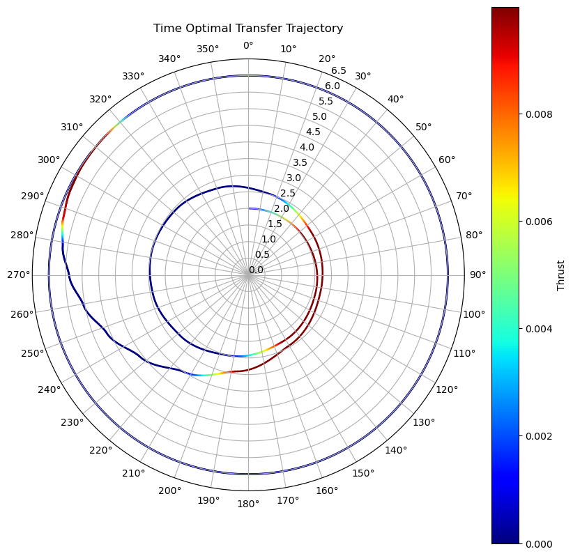
)

xxxxxxxxxx
Total number of variables............................:      481
                     variables with only lower bounds:      121
                variables with lower and upper bounds:        0
                     variables with only upper bounds:        0
Total number of equality constraints.................:      363
Total number of inequality constraints...............:      181
        inequality constraints with only lower bounds:       60
   inequality constraints with lower and upper bounds:        0
        inequality constraints with only upper bounds:      121

Number of Iterations....: 237
                                   (scaled)                 (unscaled)
Objective...............:   2.8805752505683396e-01    2.8805752505683396e-01
Dual infeasibility......:   6.4126481902349042e-13    6.4126481902349042e-13
Constraint violation....:   2.7478019859472624e-15    2.7478019859472624e-15
Complementarity.........:   2.5059035597957591e-09    2.5059035597957591e-09
Overall NLP error.......:   2.5059035597957591e-09    2.5059035597957591e-09

Number of objective function evaluations             = 291
Number of objective gradient evaluations             = 238
Number of equality constraint evaluations            = 291
Number of inequality constraint evaluations          = 291
Number of equality constraint Jacobian evaluations   = 238
Number of inequality constraint Jacobian evaluations = 238
Number of Lagrangian Hessian evaluations             = 237
Total CPU secs in IPOPT (w/o function evaluations)   =      1.249
Total CPU secs in NLP function evaluations           =      1.721

EXIT: Optimal Solution Found.
(2950,)

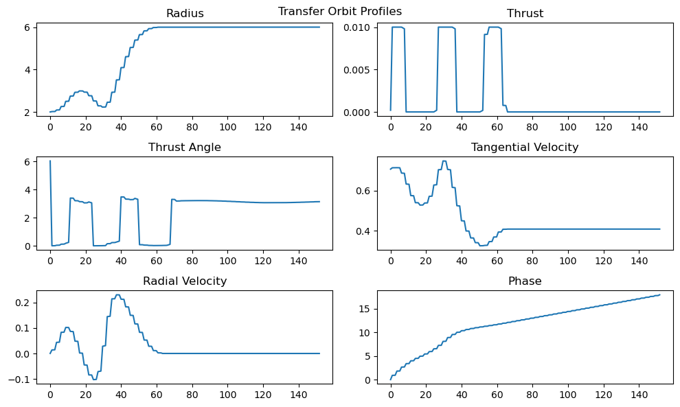
We clearly are getting a much faster time to orbit, at the cost of higher fuel usage. However, this model of the problem seems to have many local minima. This cannot be the global optimum of the model, as the model keeps running once it has reached its final orbit. If it was at the global minimum, then it would stop once it reached the final orbit.

As such, we also investigated a penalty method for finding a pseudo time optimal orbit based on the fuel optimal model.

Pseudo Time Optimal

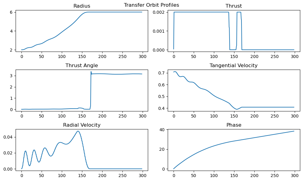
Below we use a penalty objective for the fuel optimal model that penalizes proportional to the distance the trajectory is at every time step from the final orbit radius.

xxxxxxxxxx
l = 0.0001
runHermite(
    "Pseudo Time Optimum Transfer Trajectory",
    l,
    modelObjective=pseudoTime,
    T=300.0,
    N=200,
    max_thrust=0.002,
    r_init=2.0,
    r_final=6.0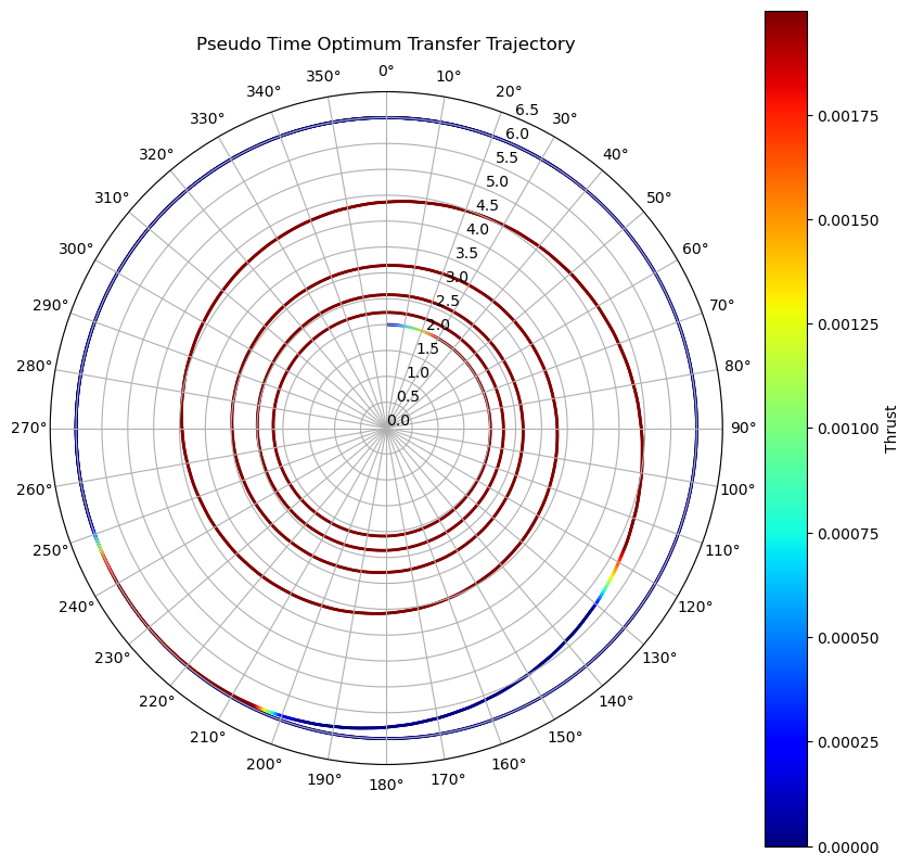
)

xxxxxxxxxx
Total number of variables............................:     1800
                     variables with only lower bounds:      400
                variables with lower and upper bounds:        0
                     variables with only upper bounds:        0
Total number of equality constraints.................:     1203
Total number of inequality constraints...............:     1000
        inequality constraints with only lower bounds:      600
   inequality constraints with lower and upper bounds:        0
        inequality constraints with only upper bounds:      400

Number of Iterations....: 110

                                   (scaled)                 (unscaled)
Objective...............:   2.2503528044705384e-01    2.2503528044705384e-01
Dual infeasibility......:   5.0723425459864302e-11    5.0723425459864302e-11
Constraint violation....:   6.5225602696727947e-15    6.5225602696727947e-15
Complementarity.........:   2.5059035607398638e-09    2.5059035607398638e-09
Overall NLP error.......:   2.5059035607398638e-09    2.5059035607398638e-09

Number of objective function evaluations             = 159
Number of objective gradient evaluations             = 111
Number of equality constraint evaluations            = 159
Number of inequality constraint evaluations          = 159
Number of equality constraint Jacobian evaluations   = 111
Number of inequality constraint Jacobian evaluations = 111
Number of Lagrangian Hessian evaluations             = 110
Total CPU secs in IPOPT (w/o function evaluations)   =      1.552
Total CPU secs in NLP function evaluations           =      0.557

EXIT: Optimal Solution Found.

We can clearly see that without the time penalty included in the objective, the model tries to get to orbit much faster by thrusting almost continuously the whole way. The details of this trajectory, and the study of different penalty multipliers hat follows, are discussed in the results section.

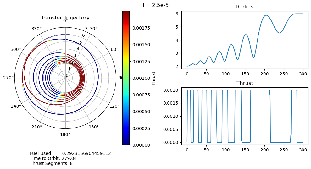
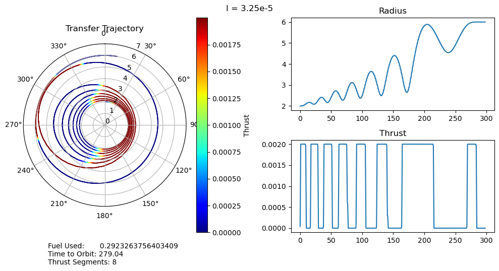
Pseudo Time Optimal

WARNING The next cell will take a bit to run. Usually takes about 3 minutes.

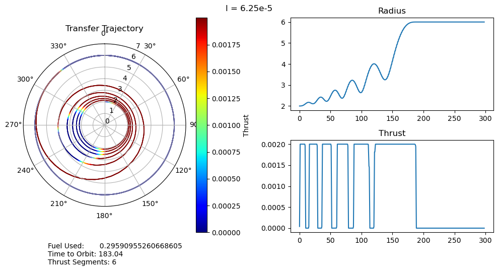
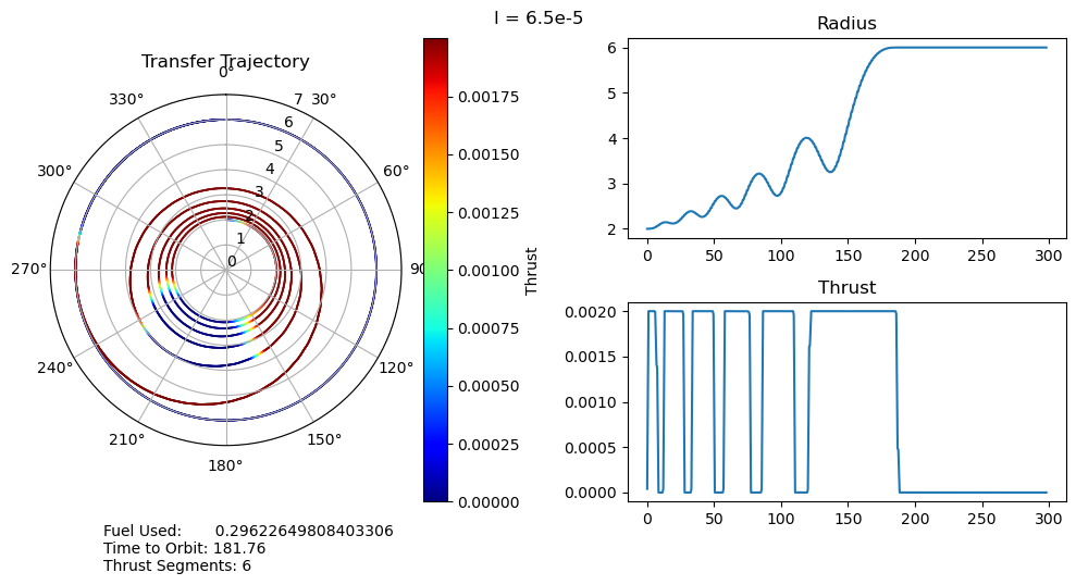
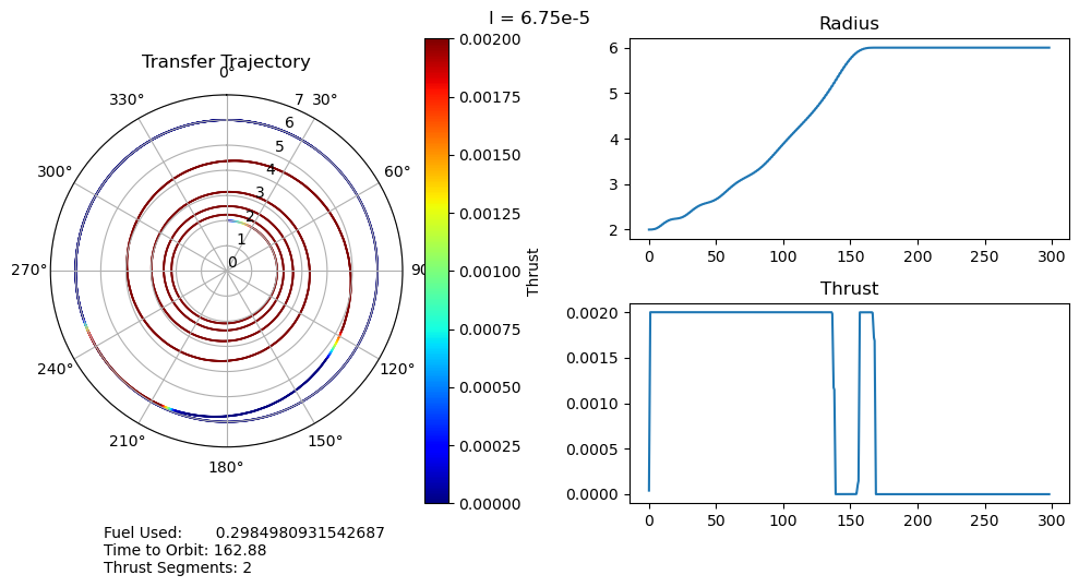
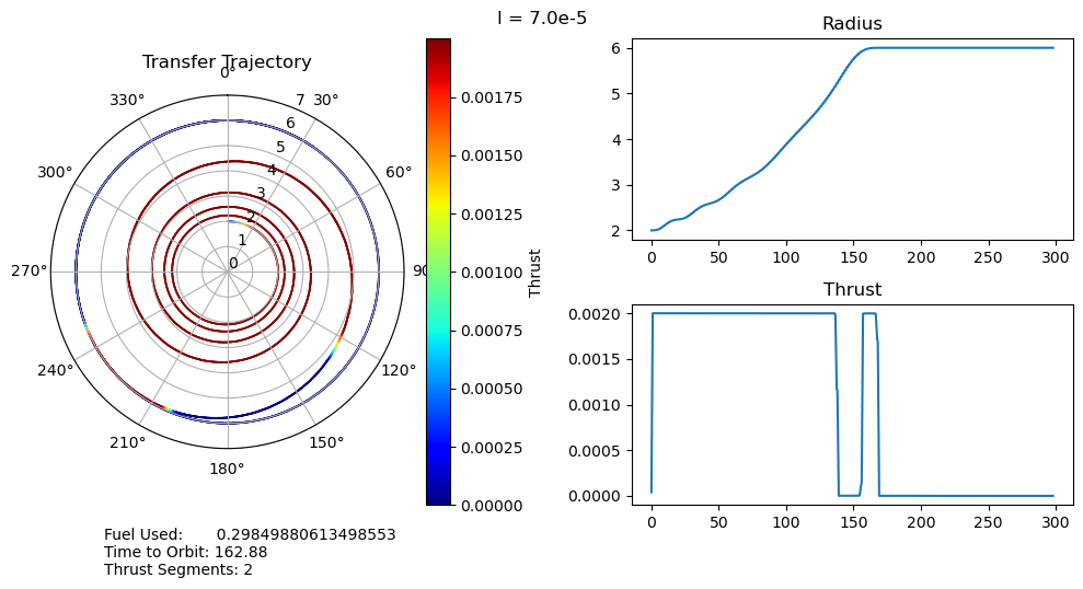
xxxxxxxxxx
# l_set = [0.001, 0.00008, 0.00007, 0.0000675, 0.0000670, 0.0000665, 0.0000660, 0.0000655, 0.000065, 0.00006, 0.00005, 0.00004, 0.00003, 0.00002]
l_set = convert(Array, 0.00002:0.00001/4:0.00008)

function pseudoTimeStudyCompute()
    all_outputs = Dict()
    for l in l_set
        output = transferOrbitHermite(
            l,
            modelObjective=pseudoTime,
            T=300.0,
            N=200,
            max_thrust=0.002,
            r_init=2.0,
            r_final=6.0
        )

        output = reconstructPaths(out_dis=output)
        
        all_outputs[l] = output
    end
    
    return all_outputs
end

pseudo_time_output = pseudoTimeStudyCompute()

xxxxxxxxxx
Total number of variables............................:     1800
                     variables with only lower bounds:      400
                variables with lower and upper bounds:        0
                     variables with only upper bounds:        0
Total number of equality constraints.................:     1203
Total number of inequality constraints...............:     1000
        inequality constraints with only lower bounds:      600
   inequality constraints with lower and upper bounds:        0
        inequality constraints with only upper bounds:      400
        
Number of Iterations....: 204
                                   (scaled)                 (unscaled)
Objective...............:   2.0349554301142975e-01    2.0349554301142975e-01
Dual infeasibility......:   4.8865356205851640e-12    4.8865356205851640e-12
Constraint violation....:   5.8564264548977008e-15    5.8564264548977008e-15
Complementarity.........:   2.5059035596999075e-09    2.5059035596999075e-09
Overall NLP error.......:   2.5059035596999075e-09    2.5059035596999075e-09

Number of objective function evaluations             = 263
Number of objective gradient evaluations             = 205
Number of equality constraint evaluations            = 263
Number of inequality constraint evaluations          = 263
Number of equality constraint Jacobian evaluations   = 205
Number of inequality constraint Jacobian evaluations = 205
Number of Lagrangian Hessian evaluations             = 204
Total CPU secs in IPOPT (w/o function evaluations)   =      3.141
Total CPU secs in NLP function evaluations           =      0.938

EXIT: Optimal Solution Found.

xxxxxxxxxx
........................ Lots of similar output later .........................

xxxxxxxxxx
ioff()

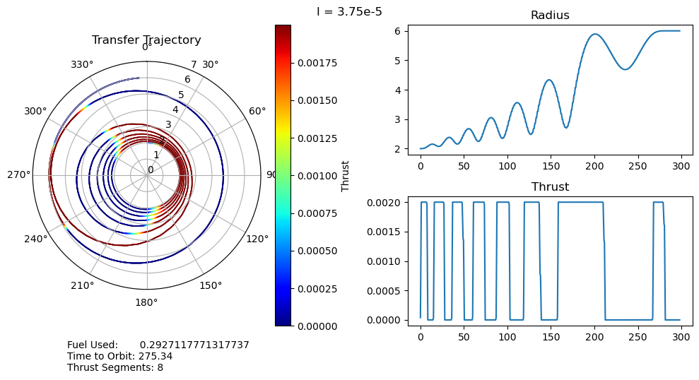
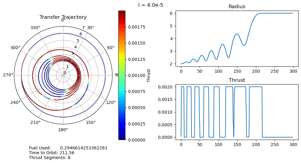
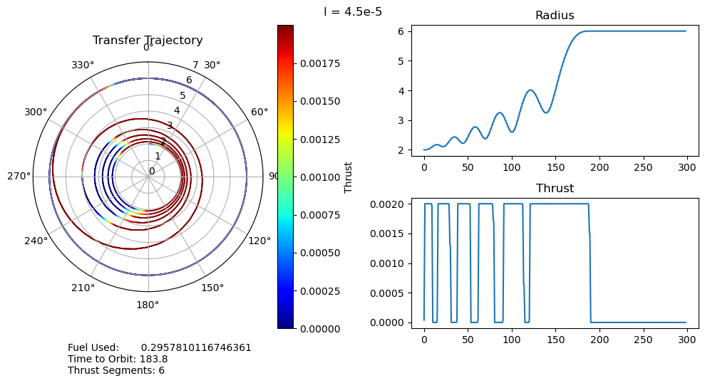
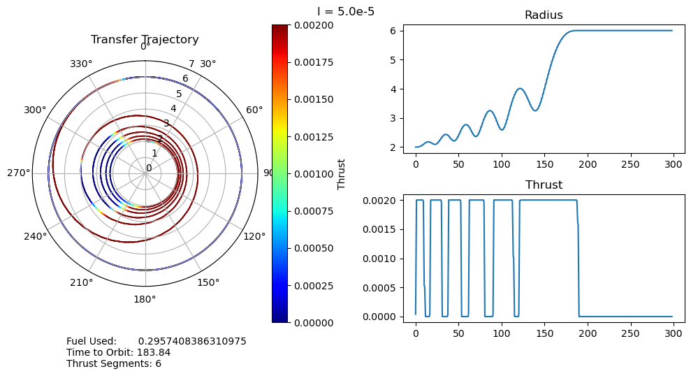
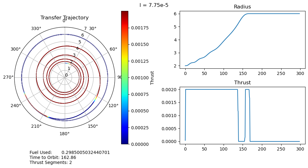
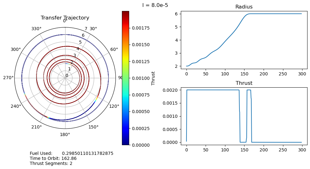
function smallOutput(;output, l, time_to_orbit, fuel_used, segments, count)
    fig = figure("pyplot_subplot_mixed$count",figsize=(10,5))
    ax = subplot(121, polar="true")
    PyPlot.title("Transfer Trajectory")
    p = scatter(output["θ"][end:-1:1], output["r"][end:-1:1], c=output["u"][end:-1:1], cmap="jet", s=0.1)

    dtheta = 30
    ax.set_thetagrids(collect(0:dtheta:360-dtheta)) # Show grid lines from 0 to 360 in increments of dtheta
    ax.set_theta_zero_location("N") # Set 0 degrees to the top of the plot
    ax.set_theta_direction(-1) # Switch to clockwise
    ax[:set_yticks](convert(Array, 0:1.0:7.0))
    color_bar = PyPlot.colorbar()
    color_bar.set_label("Thrust")
    fig.canvas.draw()
    
    subplot(222)
    plot(output["t"], output["r"]);
    title("Radius")
    
    subplot(224)
    plot(output["t"], output["u"]);
    title("Thrust")
    
    suptitle("l = $l")
    fig.text(0.1, -0.05,
        "Fuel Used:       $fuel_used\nTime to Orbit: $time_to_orbit\nThrust Segments: $segments"
    )
    fig.canvas.draw()
    fig.tight_layout()
    
#     println("Fuel Used:     ", fuel_used)
#     println("Time to Orbit: ", time_to_orbit)
end

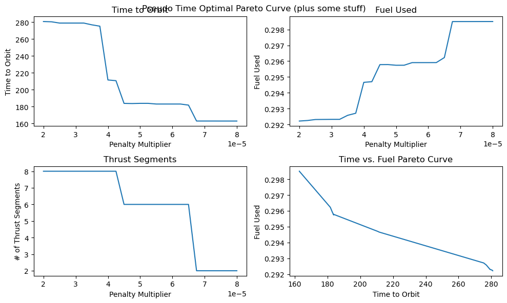
function pseudoTimeStudyAnalyze(;all_outputs, l_set)
    time_to_orbit = Dict()
    fuel_used = Dict()
    thrust_segments = Dict()
    
    for l in l_set
        time_to_orbit[l] = timeToOrbit(all_outputs[l], 6.0)
        fuel_used[l] = fuelUsed(all_outputs[l])
        thrust_segments[l] = thrustSegments(all_outputs[l])
    end
    
    count = 1
    for l in l_set
        smallOutput(
            output = all_outputs[l],
            l = l,
            time_to_orbit = time_to_orbit[l],
            fuel_used = fuel_used[l],
            segments = thrust_segments[l],
            count = count
        )
        count += 1
    end
    
    
    fig = figure("pyplot_subplot_mixed$count",figsize=(10,6))
    ax = subplot(221)
    plot(l_set, [time_to_orbit[l] for l in l_set])
    xlabel("Penalty Multiplier")
    ylabel("Time to Orbit")
    title("Time to Orbit")
    
    ax = subplot(222)
    plot(l_set, [fuel_used[l] for l in l_set])
    xlabel("Penalty Multiplier")
    ylabel("Fuel Used")
    title("Fuel Used")
    
    ax = subplot(223)
    plot(l_set, [thrust_segments[l] for l in l_set])
    xlabel("Penalty Multiplier")
    ylabel("# of Thrust Segments")
    title("Thrust Segments")
    
    ax = subplot(224)
    plot([time_to_orbit[l] for l in l_set], [fuel_used[l] for l in l_set])
    xlabel("Time to Orbit")
    ylabel("Fuel Used")
    title("Time vs. Fuel Pareto Curve")
    
    suptitle("Pseudo Time Optimal Pareto Curve (plus some stuff)")
    fig.canvas.draw()
    fig.tight_layout()
end